
Your fleet dashboard shows every vehicle's latest location, fuel level, and engine status. Yet a delivery still arrives late because the useful clue wasn't in the latest snapshot. It was in the sequence: engine temperature rose gradually, route speed fell at a recurring point, and several vehicles began idling longer than usual.
That's the practical value of time-series analytics. It turns timestamped observations into evidence about what's changing, what repeats, what looks abnormal, and what may happen next. The same approach helps an energy team understand interval consumption, an IoT operator identify equipment degradation, and a logistics manager adjust routes before service levels suffer. AWS describes these applications across demand planning, financial forecasting, and infrastructure monitoring.
Introduction to Time-Series Analytics and Why Timing Matters
A static report might tell you that a warehouse consumed more energy this month than last month. It won't tell you whether the increase happened during a particular shift, followed a change in outside conditions, or began after one cooling unit started cycling incorrectly. Those answers depend on when each measurement occurred and how it relates to the measurements before and after it.
Suppose a logistics team receives location events from trucks, temperature readings from refrigerated containers, and delivery scans from distribution centers. Looking at each event independently can confirm what happened. Ordering the events reveals the operating story. A temperature rise before a delay may indicate equipment trouble. Repeated congestion at a similar route interval may justify a dispatch change. A gap in telemetry may indicate a sensor or connectivity problem rather than normal vehicle behavior.
Operational rule: A timestamp isn't decoration. It's part of the meaning of the measurement.
Time-series analytics is designed for those sequences. It helps teams separate trend, such as steadily increasing demand, from seasonality, such as a recurring daily or weekly pattern. It also supports early warning, because a system can compare current behavior with an expected range instead of waiting for a monthly total to look unusual.
The discipline has deep roots. Time-series analytics reaches back to at least the 17th century, while its modern statistical foundations developed in the 20th century. Recursive computation in state-space models, especially the Kalman filter framework, became a major milestone beginning in the 1950s, enabling real-time estimation and forecasting from sequential observations. Earlier contributions are associated with Yule, Fisher, Tukey, Whittle, and Bartlett, alongside ideas from seasonal adjustment, leading and lagging indicators, and index numbers. This historical overview traces those developments.
The practical path is straightforward: understand the behavior of the series, store it so the structure remains usable, query it at decision-relevant intervals, then apply detection or forecasting methods that match the operational need. The outcome isn't merely a chart. It's a faster, better-supported decision.
How Time-Series Data Behaves and What Makes It Unique
Time-series data behaves more like a conversation than a pile of unrelated messages. A machine's current vibration can depend on its recent operating state. Today's demand can relate to yesterday's demand. A network's current latency can follow a sequence of congestion, retries, and recovery.
That relationship is called autocorrelation. Observations over time often aren't independent, which is the essential distinction between time-series methods and general process monitoring, as explained by the U.S. National Institute of Standards and Technology's time-series guidance.
Start with the sequence
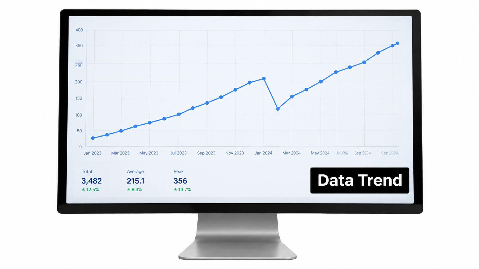
Take a stream of smart-building power readings. A single high value may be harmless if it occurred during a scheduled startup. The same value may be concerning if it appears during an unoccupied period and follows a gradual rise across several readings.
Analyze the data in three layers:
- Trend describes the longer movement. Demand may rise as a facility adds equipment, or a battery's usable capacity may decline over time.
- Seasonality describes a repeating pattern tied to a calendar or operating cycle. Heating demand may follow recurring daily behavior, while logistics activity may vary by shift or route schedule.
- Residual variation is what remains after the predictable structure has been accounted for. This layer is often where anomalies become visible.
Decomposition separates those layers so an analyst doesn't confuse a normal recurring peak with a fault. Smoothing serves a related purpose. A moving average or another smoothing method reduces short-term noise, making the underlying direction easier to inspect.
The point of smoothing isn't to erase operational detail. It's to make the signal easier to interpret without treating every fluctuation as a decision.
Why spacing matters
Regular intervals simplify comparison. If a sensor reports at consistent times, a team can evaluate changes across comparable windows. Irregular timestamps require more care because a long gap can make an apparent jump reflect missing observation rather than real behavior.
Time-series analytics also depends on the question. A maintenance team may need the latest sequence to identify deterioration. A finance team may care about recurring calendar behavior. A supply chain planner may need a longer history to distinguish a temporary disruption from a persistent shift.
That mental model prevents a common mistake: applying ordinary aggregate reporting to data whose order carries meaning. A total, average, or latest value can be useful, but it shouldn't replace analysis of the path that produced it.
Modeling and Storage Patterns That Scale
Storage design determines whether time-series analytics remains trustworthy when ingestion accelerates and operational users ask more questions. Start with a consistent event shape: an entity identifier, an event timestamp, one or more measurements, and the context needed to interpret them.
A narrow schema stores measurements as rows, often with fields such as device, timestamp, metric name, and value. It works well when devices produce different metrics or when new measurements appear frequently. A wide schema stores several measurements as columns in the same record. It can simplify queries for a stable device model, but changing the schema becomes more disruptive when the telemetry contract evolves.
Preserve time before optimizing it
Store the event time separately from ingestion time. A device may generate a reading before connectivity allows the platform to receive it. If those timestamps are collapsed, analysts can mistake delayed delivery for a change in the underlying process.
Keep the original precision needed for the decision, then create derived time keys for common access patterns. Examples include calendar date, hour, shift, route, billing period, or operational region. Partitioning and clustering should follow the filters users apply, not a generic assumption that every query starts with the same time range.
Retention and downsampling also need a business rule. Raw data may be essential for incident investigation, while older summaries can support long-term trend analysis. Keep enough detail to reproduce important decisions, and avoid deleting raw observations because a dashboard no longer displays them.
Treat compression as a performance choice
Compression affects storage consumption and the amount of data that queries must scan. Benchmark guidance for IoT and IIoT workloads reports real-world compression ratios typically in the 5:1 to 20:1 range, with advanced algorithms often reaching 10:1 or better. The TDengine benchmarking guidance also stresses that fair comparisons should measure write throughput, query latency, and compression under identical hardware and repeated runs.
Those results aren't universal guarantees. Data shape, cardinality, ordering, encoding, and workload tuning all matter. Test with representative telemetry rather than synthetic rows that omit the irregularities your operators face.
Design test: Replay realistic writes, late events, corrections, and dashboard queries before choosing a storage pattern.
For Snowflake-centered architectures, separate raw landing data from curated analytical tables. Use governed transformations to standardize timestamps, units, device identifiers, and quality flags. This separation gives analysts a stable interface while preserving a traceable path back to source events.
Query and Aggregation Strategies for Faster Insights
A good query starts with the decision, not the table. An operations manager asking, “Which assets need attention now?” needs recent detail. A capacity planner asking, “How is demand changing across the quarter?” usually needs a consistent rollup rather than every raw event.
Choose the smallest useful window first. Raw points are appropriate for incident investigation, sensor validation, and short-lived anomalies. Minute-level summaries can support control-room monitoring. Hourly summaries often fit shift and capacity reviews. Daily summaries are useful for inventory, demand, and longer trend comparisons.
Choosing the Right Aggregation Window
Business QuestionRecommended WindowWhy It WorksWhich device is behaving abnormally right now?Raw or near-real-timePreserves the sequence needed to inspect the eventDid a route or shift experience repeated delay?Shift or route intervalAligns the analysis with how managers schedule workIs facility demand changing during operating hours?HourlyReduces noise while retaining operational variationHow does consumption compare across planning periods?Daily or longer business rollupSupports trend and planning decisions without scanning every event
The table is a starting point, not a fixed rule. A battery operator may require fine-grained readings for safety review, while a finance team may prefer a calendar-aligned summary. Store or materialize the rollups that answer repeated questions, and reserve expensive raw scans for investigations that need them.
Make late data visible
Late-arriving events can corrupt aggregates if the pipeline assumes that arrival order equals event order. Track both event time and ingestion time, then define how corrections update affected windows. A delayed reading should be identifiable as delayed, not blended into the period in which it arrived.
Continuous aggregates or scheduled rollups can keep dashboards responsive, but they need quality controls. Reconcile aggregate totals with source data, monitor refresh lag, and expose whether a displayed interval is complete. SQL tools can support timestamp filters, grouping, and visual exploration, as demonstrated by Tinybird's time-series analytics workflow.
A fast query that answers the wrong interval is still a bad operational tool. Match the window to the decision, make data freshness explicit, and keep a path to raw evidence.
Anomaly Detection and Forecasting Techniques in Practice
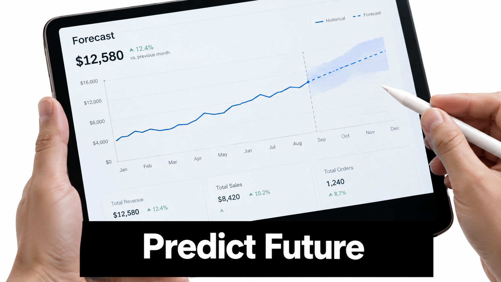
Anomaly detection and forecasting answer different questions. Anomaly detection asks whether the current observation or pattern looks unusual. Forecasting asks what the series may do next. Confusing them leads to alerts that don't support action and forecasts that are judged against the wrong horizon.
For anomaly detection, begin with an interpretable baseline. A common convention treats observations with an absolute z-score greater than 3 as anomalies. Looser settings may use 2 standard deviations, which can flag about 5% of points, while stricter settings may use 4 or higher. This practical explanation of sigma-based detection describes those common choices.
A threshold isn't a diagnosis. It identifies a candidate event for review. If a sensor's normal range changes by shift, season, or operating mode, a single global threshold can produce avoidable alerts. Compare against a suitable baseline, group related signals, and add persistence rules so one harmless spike doesn't wake an on-call engineer.
One review describes a common alert form as μ(S_T) + α·σ(S_T), with α often set to 3, tying the cutoff to the mean and standard deviation of the score distribution. The threshold discussion is available in this anomaly-detection review. Use the formula as an explainable starting point, then validate it against the cost of missed failures and unnecessary interventions.
Forecasting works differently:
- Smoothing and decomposition help when trend and recurring patterns are stable enough to extrapolate.
- State-space and related statistical models can update estimates as new observations arrive.
- Foundation-model approaches may offer broader generalization, but they require careful evaluation because temporal leakage can make a model appear stronger than it is.
Recent forecasting benchmarks emphasize zero-shot and leakage-free evaluation. Microsoft's ProbTS benchmark was introduced to unify forecasting evaluation, while GIFT-Eval tests generalization across 28 datasets, more than 144,000 time series, and 177 million data points. Microsoft's benchmark overview explains the motivation.
Judge a forecast by the decision it supports. A route planner needs a useful planning horizon and understandable uncertainty. A maintenance team needs enough warning to schedule intervention. Accuracy matters, but interpretability and decision relevance matter too.
Platform Considerations for Scale Including Snowflake Best Practices
A platform is ready for time-series analytics when it can ingest reliably, preserve event context, serve concurrent users, and explain its costs. Technology leaders should assess the complete operating path, from device or application capture through transformation, storage, query, alerting, governance, and recovery.
Evaluate the workload, not the product label
Ask these questions before selecting architecture:
- Ingestion behavior: Can the platform handle bursts, retries, duplicate events, and late-arriving timestamps without losing provenance?
- Query concurrency: Can dashboards, investigations, scheduled transformations, and forecasting jobs coexist without starving one another?
- Data quality: Can teams expose missing measurements, unit mismatches, clock errors, and corrections instead of hiding them?
- Governance: Can access policies protect sensitive location, financial, or operational data while allowing analysts to work efficiently?
- Cost control: Can owners identify expensive scans, set retention policies, and align compute with actual usage?
- Recovery: Can operators replay or rebuild derived tables when a source, transformation, or business rule changes?
Snowflake can fit this pattern when teams separate durable storage from the compute used for ingestion, transformation, exploration, and scheduled analytics. A practical design often includes a raw layer, a standardized time-series layer, and purpose-built aggregates for dashboards and recurring decisions. Snowflake's governance and workload management capabilities should be configured around the organization's access model and service expectations, not added after deployment.
Compression and clustering still require measurement. The benchmark principles discussed earlier apply here too. Test representative event distributions, query filters, concurrency, and retention behavior, then compare the result with the operational value of faster answers.
For an energy management workload, Faberwork's Snowflake time-series data example provides a relevant reference point for interval data management. Faberwork LLC is one option for organizations evaluating data transformation, integration, analytics, and Snowflake-centered time-series architecture.
A scalable platform also needs operational ownership. Define who responds when telemetry stops, who approves schema changes, which aggregates are trusted for billing or planning, and how analysts verify a surprising result. Technical scale without clear accountability produces fast confusion.
Industry Examples and Next Steps with Time-Series Analytics
The same pattern appears across industries: capture events with trustworthy timestamps, preserve the sequence, create the right rollups, and connect an observed change to a decision.
In IoT and smart buildings, operators can compare occupancy, equipment telemetry, and energy consumption across operating intervals. A building team might use fine-grained data to investigate an unexpected load, hourly summaries to review equipment behavior, and anomaly rules to prioritize inspection. A smart-building program described by Faberwork's AI transformation success story shows how time-dependent operational signals can support building optimization.
In energy, interval readings support consumption analysis, capacity planning, and operational monitoring. The important modeling choice is to preserve the meter interval and its quality status. A corrected or missing interval shouldn't look identical to a measured interval, especially when someone uses the data for settlement, planning, or equipment decisions.
In logistics, location pings, geofencing events, delivery scans, and vehicle metrics can be combined to understand route performance. Query windows should reflect route and shift operations, while anomaly detection can surface unexpected dwell time or temperature behavior. Forecasting can support demand planning, but dispatchers still need an explanation they can act on.
A practical pilot can stay focused:
- Choose one decision. Start with a concrete outcome, such as identifying abnormal equipment behavior or reducing avoidable route investigation time.
- Define the event contract. Document timestamps, identifiers, units, expected frequency, late-data behavior, and quality flags.
- Build two views. Keep a raw investigative view and a decision-ready aggregate. Make freshness and completeness visible.
- Measure usefulness. Track whether analysts find issues earlier, spend less time assembling evidence, or make planning decisions with greater confidence. Keep the measures tied to the chosen decision rather than generic dashboard activity.
- Expand carefully. Reuse the modeling and governance patterns only after the first workflow proves reliable.
The hardest production problems often involve irregular timestamps, missing values, external context, and decisions that span multiple intervals. Treat those as design requirements from the beginning. A trustworthy time-series system doesn't just predict the next value. It helps people understand what changed, why it matters, and what to do next.
If your organization is choosing a first use case, inventory the timestamped data already available, select one operational decision, and test it with representative raw and late-arriving events. Contact Faberwork to evaluate a Snowflake-centered architecture for your IoT, energy, or logistics workload and turn the pilot into a governed production workflow.


